Excel sheet as a source to Power Query and Power BI: a pitfall of UsedRange
When you import data from an Excel workbook to the Power Query or Power BI from entire sheet, be careful, there is a pitfall.
After linking to an external Excel file there are three options of data extracting available:
- From table (table-formatted range of cells in the sheet),
- From custom named range of cells,
- From entire sheet
In the first case, a Table object is already structured data with columns’ names, automatically transformed to PQ tables. In the second case, Power Query shall give the named range generic titles (Column1, Column2, etc.) and then work as before.
However, it is often the case that data are not structured in a formatted table or named range, and it can be difficult to transform them to such view before import. There can be many reasons for that, e.g., cells format is to be saved (merged cells are no longer merged after transformation) or there are too many files to transform them manually.
Data on a “raw” sheet
Fortunately, Power Query can extract data from the whole sheet. To get data from unformatted sheet you do not need to perform any special actions: just connect to the file, find the needed sheet (it will have “Sheet” value in the [Kind] column) and get data by retrieving its content from the [Data] column:
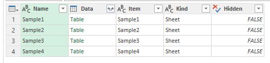
Excel sheets available as data sources just as tables or named ranges
The question is: what data range will be retrieved in that case? There are 17 179 869 184 cells on an Excel sheet (16 384 columns and 1 048 576 rows). If Power Query try to get them all, there will be huge memory consumption and performance leak. However, we can ensure that usually number of imported rows and columns is about the same as the number of rows and columns with the data may be slightly bigger.
So how Power Query defines a data range on a sheet? The answer is out there if you familiar with VBA macros and have enough experience with an Excel object model (but I think you will not be glad with this answer).
Actually, Power Query uses a special range from the sheet, named “UsedRange”.
The Unpredictable UsedRange
If you are not familiar with VBA or never work with UsedRange, there is a brief description below.
We cannot see UsedRange in the custom names list and cannot refer to it in other way except VBA. To get its address for the current active sheet, you can press Alt-F11, then Ctrl+G and write next VBA expression:
|
1 |
?ActiveSheet.UsedRange.Address |
MSDN gives us a laconic and “exhaustive” description: UsedRange is the range “object that represents the used range on the specified worksheet”. So, in other words, every used cell is included in the UsedRange. UsedRange is rectangular, so its top-left cell defined by:
- First row, which has any value, formula or format in its any cell, and
- First column, which has any value, formula or format in its any cell.
The same rule acts for the bottom-right cell:
This range includes all used cells
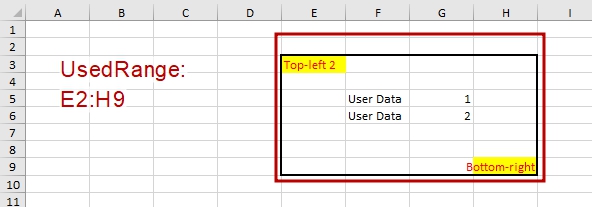
It is very hard to predict what cells Excel will count as the used range on the certain sheet. Sometimes formatting applied to the cells is invisible or implicit, and sometimes even format of the one cell can expand used range to the other row/column. For example, changing a row height can add cells to the UsedRange (but changing of column width – not).
The simplest example is: if you apply any color to the cell background (even “No Fill”!), then you can be sure that this cell is marked as used. Or, when you apply thick line to the top border of the cell, then the cell on top of the formatted one also becomes used, but if the same border line applied to left, right or bottom borders – then UsedRange don’t expand:
We just changed border line thickness, what could go wrong?
Where is the trap?
This unpredictable behavior of UsedRange has to be considered when you perform import from an Excel sheet in Power Query or Power BI. There is no problem with empty (formatted, but contain no values) rows and columns AFTER the data, but those BEFORE data are a real disaster.
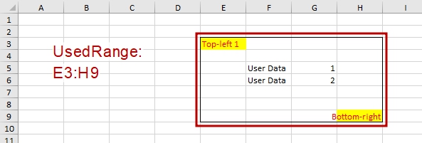
Imagine you have a few (or many) Excel workbooks, filled by different users. These workbooks have the same data structure; at least we can be sure that a range we need to extract from the given sheet is always the same. For example, desired data range is E3:H9 (four columns and seven rows). First four columns and first two rows on a sheet are empty (no values or formulas).
To get desired data, we will perform usual actions after connecting to the folder where our files are placed:
- For each file, get desired sheet,
- Keep only needed columns, from Column5 to Column8 (E:H),
- Remove first two rows
- Keep only first seven rows.
Generally, these steps do not cause big difficulties. We can write custom function or use built-in “function from the sample” feature to combine data from several sources. However, in both cases we can get discouraging results.
Starting from the second step, we are relying upon sheet structure: we need a data from 5th to 8th columns (E:H), so (we think so) we can remove first four columns. Nevertheless, UsedRange imported by Power Query may include or not include these four empty columns, depending on whether cells in them was used or not.
So, if Power Query loaded UsedRange starting from the column A, we need to remove first four columns (or select Column5, Column6, Column7, Column8 – almost the same in that case).
On the other hand, if UsedRange does not include columns 1-4, then these columns are not imported in Power Query. THEN the first loaded column is column E, where our data range begins, and we need to keep first four columns, otherwise we will remove all our data!
The same for the rows: even if first two rows do not contain any data, they will or will not be loaded by Power Query depending on UsedRange. If we always remove first two rows of data, we risk deleting important data. As a result, all following transformations will generate errors or becomes impossible.
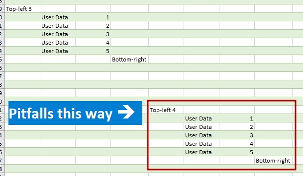
The same situation can be seen when we import data from several sheets from one workbook. I’ve prepared a sample workbook (download it here) with four sheets, containing data ranges at “E3:H9” (as on the pictures above). UsedRange on these sheets is different (you can see its addresses running a small macro in workbook):
- Sample1: E3:H9
- Sample2: E2:H9
- Sample3: E1:J12
- Sample4: A1:J13
As you can see, UsedRange on the ‘Sample4’ sheet starts from cell A1 – it means there are four empty unwanted columns/ If expanding the tables we leave only first 4 columns (As PQ will propose by default), we’ll totally miss the data from the ‘Sample4’:
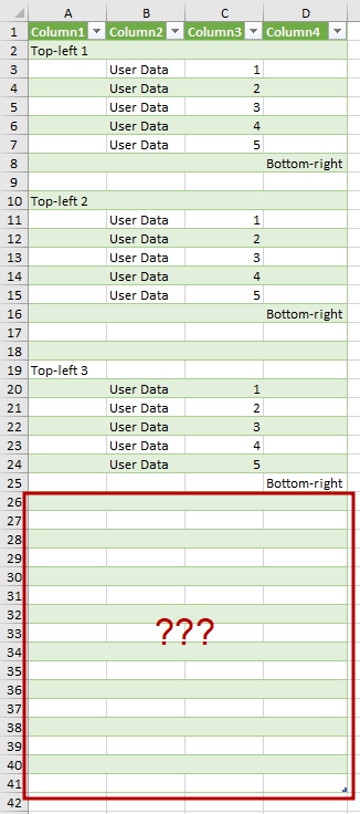
Where is the data from the 4th sheet?
If we’ll use “Load more” and retrieve all column headers, then we can see where our data migrated:
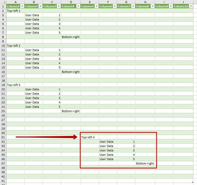
The data is not where they were expected to be seen!
You can see that not only last range moved to the right, but also there is different distance (count of empty rows) between data ranges. So how can you now explain Power Query that the desired range can be …anywhere?
Resume
Now you can see the depth of the problem. Nice if you have any attributes which allows you to recognize and locate top left cell of desired data range. However if value of this cell is dynamic (fjr example, changing date, manager name, etc.), then this task becomes almost impossible to solve in Power Query.
In any case, Power Query solution of this problem under current conditions is very hard. Even if you create custom function to check & remove first rows/columns with all null values, you cannot totally rely on it: what if a user put some data (accidentally or intentionally) in some of those columns or rows you thought to be “empty”?
As for now, there no way to explain Power Query that it need to get data from sheet starting from A1 (or other explicitly named range of cells).
If you have an option, ALWAYS format data on the sheet as a Table or as custom named range. Do not rely on import from “raw” sheet.
One relatively practical method to mark down “raw” sheets is to assign custom names to desired data ranges manually or via VBA macro. It could be done with a few strings of VBA code, but not suitable for all and in all cases (what if you cannot edit a needed workbook?).
Another trick is to place any value or format in A1 cell: you can write a small macro to check UsedRange and apply changes to A1 so it will be included. But this is nothing more than duct tape for such great tools as Power Query and Power BI.
I consider the use of UsedRange to define an imported range as an error. This is a bug, not feature. Power Query does not work with formats; there is no sense to rely on UsedRange.
In my opinion, Power Query have to import data from a “raw” sheet starting from A1 cell and up to the crossing of last non-empty column/row. In that case we can rely on address of top left cell of desired data range. Or even better, there have to be an option to pass desired range (or its top left cell) as an argument for worksheet connection. Any of these solutions will be MUCH better than what we have now.
PS. If you want to dive deep into Power Query and Data modelling, I highly recommend these excellent books:
Share this: