There are plenty examples on how to unpivot nested tables (some brilliant ones can be found here and here). But what if a table we need to make flat has no nested headers for repeating groups of columns? It ought to be nested, but it doesn’t. And standard unpivoting methods then do not works then.
Stacking (or unpivoting) non-nested groups of columns is not a common task, but sometimes it appears. It could be due to bad constructed software report or hand-made user table in Excel or web-page scrapping. But in some case, we meet with this horror.
Once a client asked me to help with intelligence on his database. Of course, I agreed. But when I saw this “database” which he proudly presented to me, I was glad that the customer does not see my face and did not hear any comments passed my lips.
There was an Excel worksheet with more than 100 (one hundred) columns with more than 10000 rows, with all diversity of data in it. About 80 columns was in repeating groups, named “Date”, “Sum”, “Date”, “Sum” …. “Date”, “Sum” – without nesting or grouping.
For some reasons, when a VBA solution couldn’t be applied (especially if you work in Power BI and want to pull data in it without voodoo dances), the only way to flatten this table was using the Power Query for Excel 2010-2013 (or “Get Data” in Power BI, “Get & Transform” in Excel 2016).
Working on that task I discovered that there are at least four ways of doing it. You can choose the method that best suits your case.
As-is and to-be
What we have in source and what we need to get shown on the picture below:
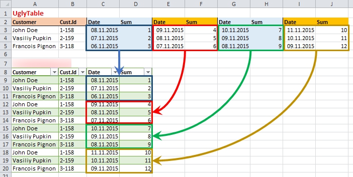
The source and the target: not so easy…
Actually we need to stack repeating groups one under other, keeping in place the common data from first columns.
Continue Reading →
Follow me: 


In my previous post I described how to pull a single value from one column and apply it as a new column’s value for specified rows. This kind of transformation could be applied when we have a mixed data source: one part of data is in a tabular form, and other part of data forms headers for these tables.
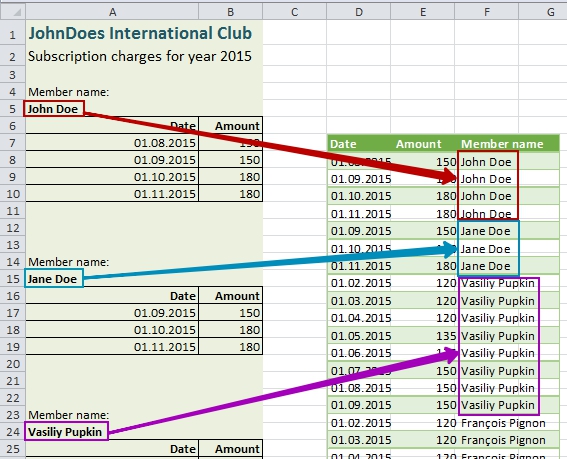
Now there is more complex task: we have a several values in separate rows, which (being taken together) form unique header for each data table. And the question is how to transform this header into new columns for tabular parts.
What we need to do is best illustrated by the picture:
What we have to do: attach title fields to data rows.
Continue Reading →
Follow me:
In my work I often meet data sources with a mix of tabular data and other useful info outside the tables. Usually it comes from some web reports or accounting programs output, where applied report criteria or other important data forms a header rows of report. While it is not so hard to make-up this data in Excel, it is better to avoid hand-made rinsing and washing every time we got a raw source updates. This becomes even more relevant when working with Power BI, where we don’t want or cannot make data preparation in Excel.
So here comes the cavalry Power Query with its outstanding abilities of raw data transformation.
(I really don’t sure how I should name this post)
The short preamble (“A long time ago…”)
You can imagine (and this is true!) that in almost every culture exists John Doe. Somehow these guys decide to unite and form a “JohnDoes International Club”. We do not know, what aims and goals of this club is (hope it is not “rule the world”), but anyway, this club exists with all necessary bureaucracy.
Every month club members have to pay membership charges. And every month club cashier got a report on charges collection.
The case
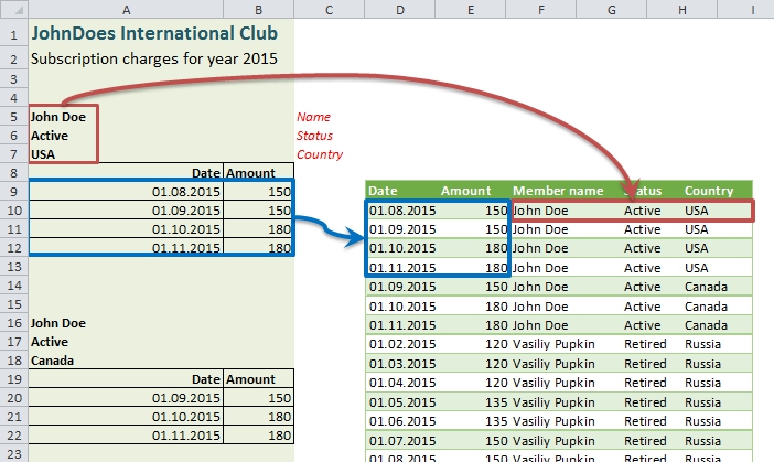
In this report we can see a standard header of what this document is about, and then information on each member’s charges. Each club member has own “table of charges” in this report, and each table precedes with two rows: pointer “Member name” and a member’ name itself.
In a sample report we can see four names: John Doe and Jane Doe form the USA, Vasiliy Pupkin from Russia and Francois Pignon from France (my apologies to monsieur Francois Dupont, but for me monsieur Pignon is already №1 due to beautiful comedies with Pierre Richard). Also please note that any coincidences to real people and clubs are accidental.
What we have to do is to make a flat table from the report:
Transfer values to a new column: things to do
Continue Reading →
Follow me:
PowerQuery is a great instrument that can do much more than just take data from source and pull it in a table or Power Pivot. We can clear and transform data in multiple ways, but there are some transformations, usual in Excel, which are not so convenient to make in Power Query.
For example, what if I need a relative reference to a specific “cell” (a value from exact row in exact column) in a PowerQuery table? Or reference to a value that is in specified column and 4 rows above from referencing row? In Excel this is obvious, I need just point on it with mouse, ensure that I removed “$” (absolute) signs from row part of reference, that’s all. But in PowerQuery I can’t do this so easy.
But anyway, a solution, still obscure, is reachable.
First of all, let’s found how we can access a particular value from a Power Query table.
The easiest way to understand item addressing in Power Query, in my mind, is analyzing of steps code.
Absolute row references
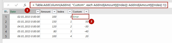
Suppose we have a simple table of two columns, “Date” and “Amount”. It has 5 rows, and in the first column it filled with, suddenly, dates, in second – some values:
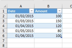
Source table
We would like to get a value from cell B4, exactly 120. Continue Reading →
Follow me: