Using the header of the report as the data for table columns in Power Query
In my previous post I described how to pull a single value from one column and apply it as a new column’s value for specified rows. This kind of transformation could be applied when we have a mixed data source: one part of data is in a tabular form, and other part of data forms headers for these tables.
Now there is more complex task: we have a several values in separate rows, which (being taken together) form unique header for each data table. And the question is how to transform this header into new columns for tabular parts.
What we need to do is best illustrated by the picture:
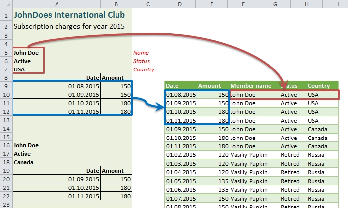
What we have to do: attach title fields to data rows.
You can see that the report that we need to convert, composed of several tables with different number of rows (this prevents us from using a trick with a column index for grouping rows). Each table is preceded by a header of several rows. These rows form the unique header, but at the same time, individual values in them are not unique and may be repeated in the headers of other tables.
As usual, there are more than only one solution of this task: we can use VBA, we can use Excel formulas, but we want to use Power Query (“Get & Transform” in Excel 2016 or query editor in Power BI Desktop). And yes, we can do it in Power Query without one hand-made “M” language code line – just with UI.
The source
The sample workbook for this case can be downloaded here.
To make a story from this case, let it be a monthly members’ charges report for the mysterious “JohnDoes International Club”. This report differs from the same in previous post with not only extended header, but also Jane Doe was replaced to John Doe from Canada to make duplicates in the original data.
I will do all transformations in the same workbook and that’s why I use a named range “ChargesExt” to refer to a data on the sheet.
But if you don’t want to add named ranges, you can make a query from another workbook to an Excel file (if you make a query from Power BI, it is almost only way). Then you need to drill not to the named range, but to a sheet in this file.
The other way is to change original source sheet by creating an Excel table on it, but I don’t like it. Let the source be untouched.
Prerinsing
First of all, we need to prepare data by removing all unnecessary info.
- Open Power Query editor with empty query.
- Enter = Excel.CurrentWorkbook() in formula bar (I lied: this is the only formula you need)
- Drill to table named “ChargesExt”
- Remove empty rows
- Remove two first rows (report header)
- Add Index column
Now we have a little bit washed table, and can start a real transform from here:
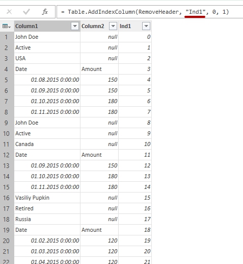
A little bit wahsed source
Note that I changed automatically generated name of “Index” column to “Ind1” manually editing formula of this step, but it is not necessary.
Name this query as “CleanExt” and then “Close & Load to… -> Create connection only”
Transformation
My plan to make all necessary transformation is simple and kind of similar to trick from previous post:
- create a column of only headers rows,
- add special repeating index column (0,1,2,0,1,2,…,0,1,2 etc.)
- pivot this index column to new columns
- Join this new pivoted table to our “CleanExt” query
- Make final mash-ups
But how to combine these two queries? Which column must be specified as a binder, so then we can definitely attribute “header” to the appropriate table?
In fact, the sole feature, determining the relative position of each “header”, is the row number that can be assigned to the relevant part of the report. That’s why we added index column to the “CleanExt” query.
So in the new query we need to save at least one row number for each “header”.
Let’s start:
- Right-click on “CleanExt” query in “Workbook Queries” panel and create a linked query.
- First of all, remove all “non-headers” applying filter to the “Column2” by select only “(NULL)” values.
You can see the result here: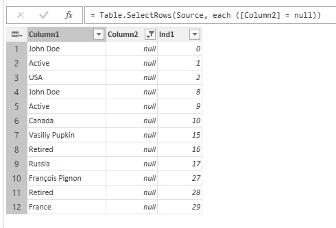
Leave only tables headers
- Add one more “Index” column: we need it for pivoting.
Select newly created “Index” column, go to “Transform” menu and in “From Number” part click “Standard” and apply “Modulo”. The idea is in creating a special index that will help us identify row positions in the header: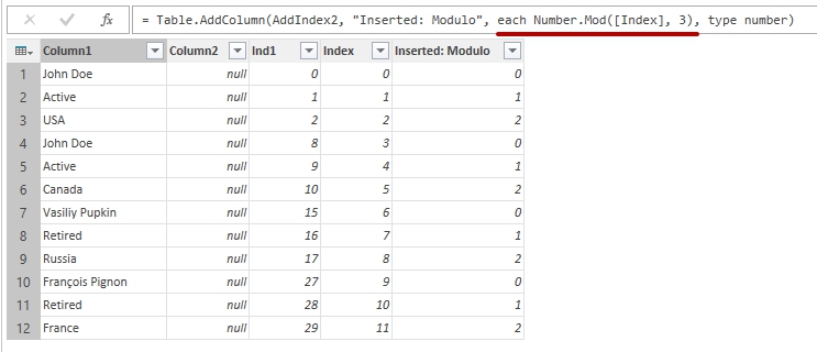
Inserted Modulo helps us pivot headers to separate columns
- Remove “Index” and empty “Column2”
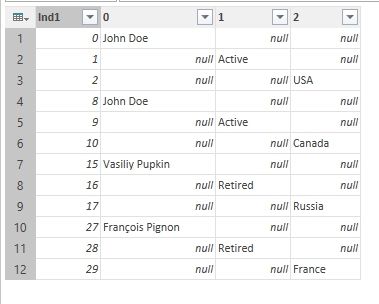
Now we have all we need to perform pivoting: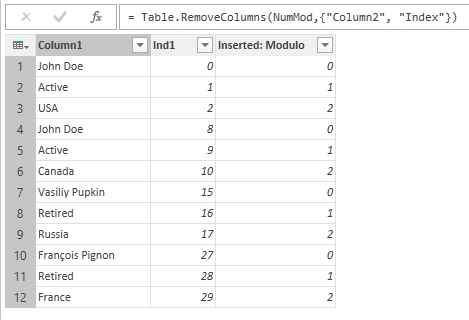
All we need is here: headers rows, row numbers to link and modulo to pivot
- Select last column and pivot it!
Header rows pivoted by its positions
- Select newly created columns “1” and “2” and go to Transform – Fill Up.
- Remove rows we don’t need any more: apply filter to column “0” by unchecking “(NULL)” values:
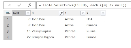
All is ready to combine two queries
Now it is ready to be combined with our source query “CleanExt”.Name this query as “HeadersTransposed”, go to Close & Save to… -> Create connection only
- On the “Workbook queries” panel right-click on “CleanExt” query and select “Combine”
- Choose “CleanExt” as first query, “HeadersTransposed” as second, and select column “Ind1” in both of queries. Press OK
- Now we got a new column to our “CleanExt” table:
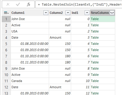
Queries combined and tables merged by row number
If you click next to green “Table” word in new column, you can see that to each first row of each “header” connected a table of 3 columns, and, as it linked by the same index number, it connected correctly.
Make-Up
- Remove “Ind1” Column
- Expand “NewColumn” by clicking on two-way arrows near its header.
- Select columns “0”, “1”, “2” and do Transform – Fill Down
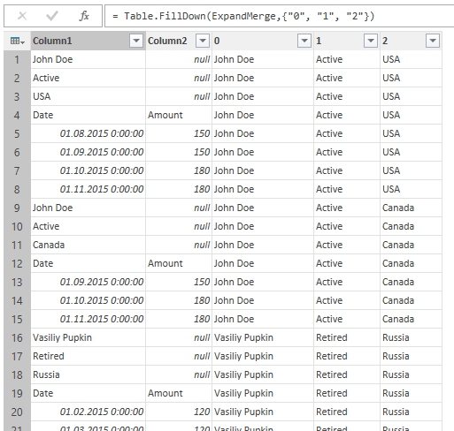
Rows filled down with all necessary data for each table
- Remove now useless header rows by applying filter to “Column2”: uncheck “(NULL)” and “Amount” in filter options.
- Rename columns to “Date”, “Amount”, “Member name”, “Status” and “Country”
- Change data type in each column before loading it to a sheet.
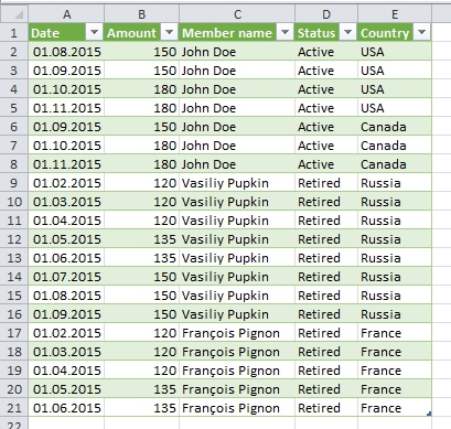
Is it what we want to get?
That’s all. I named this query as “ChargesExtByIndex” and “Close & Load” it ot a sheet.
I hope you find this trick (with row number to combine queries) interesting and inspiring, as it was for me when I “invented” it (sure not the first, but myself)
PS: In the sample workbook you can also find another query, named “ChargesExt R1C1”. This is my exercises with relative row references in Power Query to perform such transposing without merging two queries. It is Excel-style approach, which can be used on not-so-big data sources (it could cause resource consuming operations when applied to a big data sets). I find it also very interesting.
Follow me:Share this: