Faster Than Joins! Power Query Record as Dictionary: Part 3
Lookup records could be significantly faster than Left Join in Power Query, and there are three different way to create them
Continue Reading →Lookup records could be significantly faster than Left Join in Power Query, and there are three different way to create them
Continue Reading →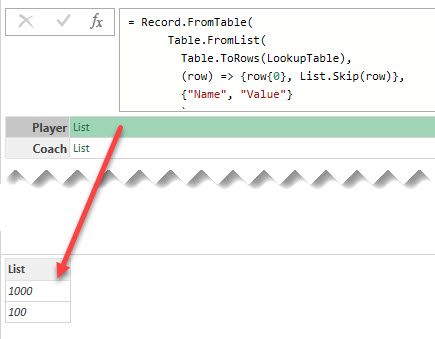
Using the Record.FieldOrDefault function in Power Query to lookup values from dictionary record and handle missing keys
Continue Reading →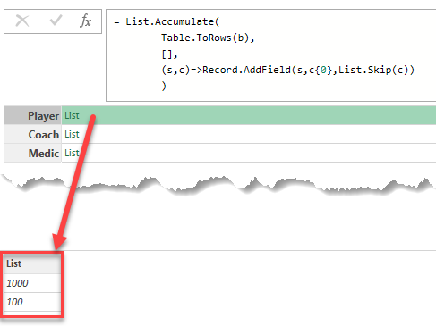
How to use a special dictionary record for a performant lookup for values in Power Query
Continue Reading →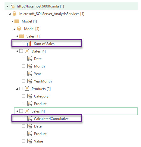
We can connect almost any data source in Power Query, but PowerPivot data model is not included in that extensive list of sources out of the box.
But with the help of the fabulous DAX Studio we can do it (although in my opinion it is still inconvenient and tricky) at least locally – from the same workbook in Excel or from Power BI Desktop.
All you need is to open your Excel workbook, run DAX Studio add-in and connect it to this workbook. Then you can just connect to the PowerPivot model as to SQL Server Analysis Services cube.
But this is an undocumented and extremely limited feature not supported by Microsoft, which can only be used under your own risk.
Continue Reading →Follow me:Let’s say you have a few numerical columns [A], [B] and [C] in your table and want to sum them to the new column in Power Query or Query Editor in Power BI.
In Power Query we have special buttons for this:
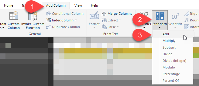
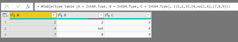
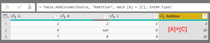
For example, we want to sum columns [A] and [C]. Just click (holding Ctrl button) column headers you want to sum, then go to “Add Column” – “Standard” – “Add”, and you’ll get a new column named “Addition” with the row-by-row sum of desired columns:
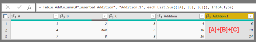
If we want to add three columns at a time, then we’ll also get a desired result:
But if in this table we want so sum columns [A] and [B], we are not expecting a pitfall, aren’t we?
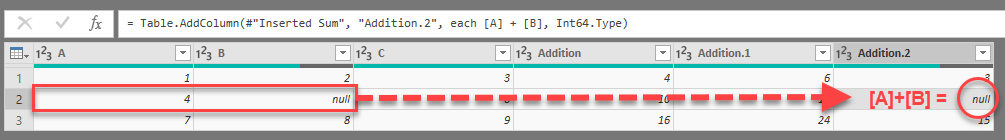
The reason of this behaviour is simple and it reveals itself when we look at our data a little bit close: there is a null in column [B] in that row. In Power Query formula language (M) the expression null + value always returns a null (see this excellent post of Ben Gribaudo about null type and operations with null values).
But why we get a correct result when we sum up three columns? It is because Power Query uses different formulas when we sum two columns or three and more columns:
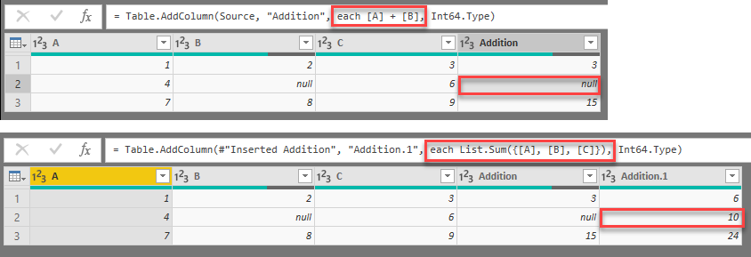
List.Sum function used in this case ignores null values and sums up only numerical values. Indeed, it gives more intuitive result, but on the contrary has not such intuitive syntax of simple addition.
I do not know what is the reason of such difference, and already complained to the development team. But if you rely on the buttons there, then you have to be aware of such behaviour.
What is the possible solutions there? It depends on what you want to get as a result, but in any case you should take a look at the formula bar and decide what to correct there:
value + null = null, then you should use simple + symbol between column names. value + null = value, then you should use List.Sum finction, like in that example: List.Sum({[A], [B], [C]})THE SAME BEHAVIOR Power Query shows when you’ll try to multiply two columns and three or more columns: with two columns there will be the simple * symbol, with three or more columns there will be List.Product function used.
Ok, it is a really short post which I planned to (and ought to) write a long time ago…
Follow me:Recently I needed to do the very simple thing in Power Query. I have the column of numbers and need to check if the values in this column are less than N and then put a corresponding text value in the new column. The function for the new column is something like this:
|
1 |
= if [Values] < 5 then "A" else "B" |
Actually some values are not a numbers but nulls:
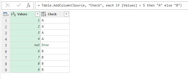
Data contains nulls and comparison return an error
And this simple calculation returns an error for these values!
Why? There is the catch, which is hidden in the depth of documentation (actually on the page 67 of the “Power Query Formula Language Specification (October 2016)” PDF which you can obtain there.
Continue Reading →Follow me: ![]()
![]()
![]()
![]()
This is a very short post, just to make a reminder and possibly expand knowledge for me and my readers.
Sometimes, specially when working with calendar tables, we need to calculate ISO Week Number for certain date. There is no native functions in Power Query / M language / Power BI to get ISO Week number, so to obtain the desired result you need to write your own function.
Thanks to Catherine Monier, Microsoft Excel MVP, for providing the link to the “Date to ISO Week” M function already written for us. There also another function for converting ISO Week date (format input like: 2017-W02-7) to the normal date:
This function is not so hard to develop, I think, but it is always better when somebody gives you ready-to-use solution, isn’t it? 🙂Follow me: ![]()
![]()
![]()
![]()
List.Generate is the powerful unction of M language (the language of Power Query aka “Get & Transform” for Excel and Power BI query editor), used for lists generation using custom rules. Unlike in other list generators (like List.Repeat or List.Dates), the algorythm (and rules) of creation of successive element could be virtually any. This allows to use List.Generate to implement relatively complex get & transform tasks.
Although there are few excellent posts about this function uses (for example, Chris Webb, Gil Raviv, PowerPivotPro, KenR), I always I always lacked a more “clear” description — «How it actually works?» or «Why don’t it work?» and, at last, «What did the developers kept in mind when create this function?»
As usual, MSDN help article is laconical:
Generates a list of values given four functions that generate the initial value initial , test against a condition condition , and if successful select the result and generate the next value next . An optional parameter, selector , may also be specified.
Will you receive a list of four elements? Do you want to use an optional selector? Really? Why not?
In abandoned Power Query Formula Reference (August 2015) we can find the more clear description:
Generates a list from a value function, a condition function, a next function, and an optional transformation function on the values.
At least it is obvious that this function takes 4 arguments, all of type function:
|
1 |
List.Generate(initial as function, condition as function, next as function, optional selector as nullable function) as list |
Actually List.Generate uses quite simple loop algorythm. When creating an element of a new list, List.Generate evaluates a some variable (lets call it CurrentValue), which then passed from one argument-function to another in a loop:
As you can see from this not-so-technical description, the important difference of List.Generate from other iterator functions of M language is that almost all of others working in “For Each…Next” style (they have a fixed list to loop over), while List.Generate uses other logic – “Do While…Loop”, checking the condition before loop iteration. Subsequently, the number of elements in created list is limited only with “While” condition.
If we’ll write down the algorithm described above in other, non-functional language (like Visual Basic), it will look like that:
|
1 2 3 4 5 6 7 8 9 10 11 12 |
Dim NewList As New List CurrentValue = initial() Do While condition(CurrentValue) If selector = null Then NewList.Add(CurrentValue) Else NewList.Add(selector(CurrentValue)) End If CurrentValue = next(CurrentValue) Loop |
Please note:
When you create a list using some API calls (for example, you send GET or POST requests to API in initial and next functions), you should consider the following:
It is convenient when both initial and next return value of type record. This greatly simplifies the addition of counters and passing additional arguments for these functions (for example, one of record fileds is main data, second is counter, etc.).
Resuming, List.Generate is the powerfull tool, looking more complicated than in fact. Hope this post made it more friendly and comprehensible. 🙂
Follow me: ![]()
![]()
![]()
![]()
Recently I posted about UsedRange trap when importing from Excel sheet in Power Query (you can read this post there).
To add an option for users who can meet the same problems as me I’ve added corresponding Power Query improvement ideas on excel.uservoice.com and https://ideas.powerbi.com
Please add your votes to these improvements – I’m sure they can not only save you a few rows of code but also can save you from potential pitfalls when working with raw Excel data.
Thank you!
Follow me: ![]()
![]()
![]()
![]()
When you import data from an Excel workbook to the Power Query or Power BI from entire sheet, be careful, there is a pitfall.
After linking to an external Excel file there are three options of data extracting available:
In the first case, a Table object is already structured data with columns’ names, automatically transformed to PQ tables. In the second case, Power Query shall give the named range generic titles (Column1, Column2, etc.) and then work as before.
However, it is often the case that data are not structured in a formatted table or named range, and it can be difficult to transform them to such view before import. There can be many reasons for that, e.g., cells format is to be saved (merged cells are no longer merged after transformation) or there are too many files to transform them manually.
Fortunately, Power Query can extract data from the whole sheet. To get data from unformatted sheet you do not need to perform any special actions: just connect to the file, find the needed sheet (it will have “Sheet” value in the [Kind] column) and get data by retrieving its content from the [Data] column:
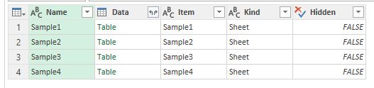
Excel sheets available as data sources just as tables or named ranges
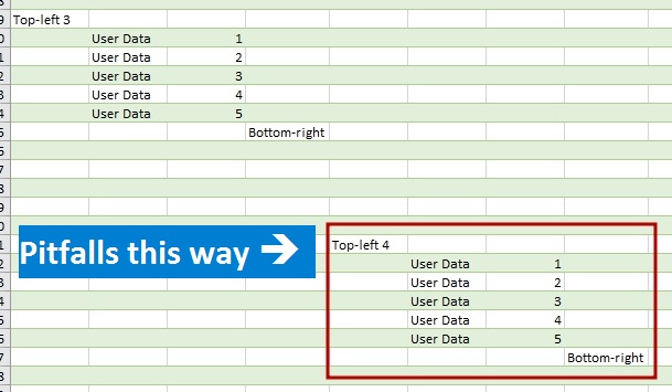
The question is: what data range will be retrieved in that case? There are 17 179 869 184 cells on an Excel sheet (16 384 columns and 1 048 576 rows). If Power Query try to get them all, there will be huge memory consumption and performance leak. However, we can ensure that usually number of imported rows and columns is about the same as the number of rows and columns with the data may be slightly bigger.
So how Power Query defines a data range on a sheet? The answer is out there if you familiar with VBA macros and have enough experience with an Excel object model (but I think you will not be glad with this answer).
Continue Reading →Follow me: ![]()
![]()
![]()
![]()