Absolute and Relative References in Power Query: R1C1 Excel-style approach
PowerQuery is a great instrument that can do much more than just take data from source and pull it in a table or Power Pivot. We can clear and transform data in multiple ways, but there are some transformations, usual in Excel, which are not so convenient to make in Power Query.
For example, what if I need a relative reference to a specific “cell” (a value from exact row in exact column) in a PowerQuery table? Or reference to a value that is in specified column and 4 rows above from referencing row? In Excel this is obvious, I need just point on it with mouse, ensure that I removed “$” (absolute) signs from row part of reference, that’s all. But in PowerQuery I can’t do this so easy.
But anyway, a solution, still obscure, is reachable.
First of all, let’s found how we can access a particular value from a Power Query table.
The easiest way to understand item addressing in Power Query, in my mind, is analyzing of steps code.
Absolute row references
Suppose we have a simple table of two columns, “Date” and “Amount”. It has 5 rows, and in the first column it filled with, suddenly, dates, in second – some values:
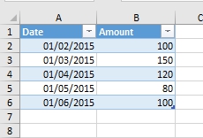
Source table
We would like to get a value from cell B4, exactly 120.
In Excel it’s easy – we just write a reference like =B4, or =R4C2 in R1C1 style.
Can we use this reference style in PowerQuery? Yes.
Load this table in Power Query, right-click on desired value and “drill to details”. Okay, we got 120.
Now take a look to code:
|
1 2 3 4 5 |
let Source = Excel.CurrentWorkbook(){[Name="Tab_1"]}[Content], Amount = Source{2}[Amount] in Amount |
In third row of code we see desired reference. Note that we refer to a previous step (as usual), then we got {2} and then – column name [Amount].
Important: rows and lists in Power Query have so called zero-based index: first position in list always has index of 0, same for the row numbers in a table. So when we ask Power Query for value from third row, we have to use 2 as row position.
This formula could be decrypted as follows: give me a value from [Amount] field in 2nd record from Source table. In other words, formula looks for specified record number inside table, and then return a specified field’s value from this record.
Formula that we get from editor actually uses two consecutive approaches:
Name{Argument} expression and
Record[Field] expression.
Actually, this Name{Argument} syntax has several implementations:
- if Name is a list and Argument is a number, expression returns the item of Name list at specified position;
- if Name is a table and Argument is a number, expression returns a row at specified position from Name table;
- if Name is a table and Argument is a record, expression returns the unique row from table Name that matches the field values of record Argument for field names that match corresponding table-column names.
Last option listed above adds a lot to imagination of what we can do with it, but now we looking straight to our question: absolute and relative references to a single value.
A Record[Field] expression has relatively same syntax: it looks up a field in a record by field name. If the specified field does not exist in the record, an error is raised.
Look at our formula again: first, we get a row (record) from Source table at position 2:
|
1 |
Source{2} |
Then we get a field [Amount] from this record (row of table is a record with column names as field names):
|
1 |
Source{2}[Amount] |
Looks easy, yes?
But wait, if we ask PowerQuery to give us a single column from table, we’ll got exactly the list:
|
1 |
MyList = Source[Amount] |
So, if we want to get a specific value from that list (see (1) above in Name{Argument} description), we just add a position number in braces next to the list name:
|
1 |
MyValue = MyList{2} |
We can shorten this two steps in one:
|
1 |
MyValue = Source[Amount]{2} |
and get desired value of 120.
So actually we have two possible ways to reach single value from a Power Query table.
Let’s compare two item addressing versions:
- Look to a specific record in a table and get a specific field from this record: MyValue = Source{2}[Amount]
- Get a list from table column and get a value from specific position in this list: MyValue = Source[Amount]{2}
It looks so similar and can give us confidence that there is no difference between column name and position order. Actually those are different approaches, and we need to remember it for future purposes.
But anyway, both this approaches are giving us a key to any type of row references in Power Query tables.
Relative row references
In sample table we have data that looks like account remnants. Suppose we need to get a calculated column which will show us a dynamic change of account values. For this purpose, we have to get a value from row above, and compare it with the value in current row.
But in previous examples we can see that position reference and column reference is hard-coded into formula. So we have to find a way to transform row numbers to relative-style reference.
And here Excel comes to help us (again). What we’ll do in Excel to make this kind of calculation? In simple way, we just put a formula in C3: =B3-B2
and fill column with it. But let’s write this formula in R1C1 style: =RC[-1]-R[-1]C[-1]
Which means “take value from this row and one-column-to-left and subtract a value from one-row-up and one-column-to-left”. In most cases in PowerQuery we will operate with values from known columns, and now let’s imagine that we can omit the part relating to the column and use only R1-style reference: =R–R[-1]
Ok, that it is. We need to get row number for current row and calculate a number of row above, so we then could use formula in one of this kinds:
|
1 |
= Source{current_row_number}[Amount] - Source{current_row_number-1}[Amount] |
or
|
1 |
= Source[Amount]{current_row_number} - Source[Amount]{current_row_number-1} |
So, is there a way to get a row number in PowerQuery? Yes. It is special Index column.
Index column generates a list of integer values, starting from N and with step S, for each row in a table. Power Query UI allows us select one of two most popular indexes: “From 0” (default) and “From 1” (both have incremental step 1), or design our own list with custom Start and Step parameters
Ok, let’s add the “Index” column (from 0) after our Source step in Power Query:
|
1 |
#"Added index" = Table.AddIndexColumn(Source, "Index", 0, 1) |
Now we have all we need: we know a column name and can get a row number from “Index” column. Let’s rename previous step to “AddInd” (so we could write it fast) and add a custom calculated column with entering this formula in dialog window:
|
1 |
=AddInd[Amount]{[Index]}-AddInd[Amount]{[Index]-1} |
This gives us full formula for this step looks like this:
|
1 |
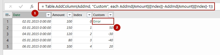
= Table.AddColumn(AddInd, "Custom", each AddInd[Amount]{[Index]}-AddInd[Amount]{[Index]-1}) |
What we just do is refer to a value from column “Index” in each row as an argument to Name{Argument} expression.
Actually, in this example I used list-position style of reference (1) against table-record style (2). Look at result in PowerQuery preview window:
Here we can see how a relative row reference works in Power Query
We got a desired list of Amount increments, but also got an error for the first row. Of course, there is no rows with position of (0-1)=-1. If we probably could use {position} bigger than last row index, then we should use “?” (a question symbol) after position reference. It called “optional item selection”.
Let’s see how it works. Go one step back and add another custom column with this formula:
|
1 |
=AddInd[Amount]{[Index]+1}? |
And what we got is:

“Optional Item Selection” returns null if we exceed row counts
i.e. reference to non-existing position in list was replaced with null value. But, as I told before, it works only with positions equal or bigger than count of items in list (or of records in table). For negative position number formula generates an error.
Ok, lets remove this step and return to previously added custom column, which has an “Error” value in first row.
What we can do with this error? We can add another step with UI: replace errors. Just select our Custom column, then Transform-Replace errors…, and put 0 in dialog window. Or just add this formula in the editor:
|
1 |
RemErrs = Table.ReplaceErrorValues(AddCust1, {{"Custom", 0}}) |
Ok, we’ve got what we want:
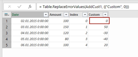
Now we rapleced errors with specific “hard-coded” values
If we would like to replace errors not with exact values but with some other calculations or functions, it is better to use “try-otherwise” construction (it works like IFERROR function in Excel). We just need to edit previous step (when we added first custom column). Click on “gear” right to the step name and replace the formula with this:
|
1 |
try AddInd[Amount]{[Index]}-AddInd[Amount]{[Index]-1} otherwise 0 |
or make necessary corrections directly in formula bar. There could be any expression after “otherwise” operator, for example, you can use custom function, enter a text o return null value.
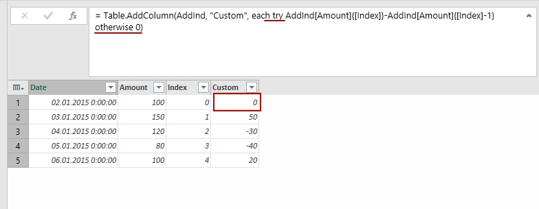
Now we replaced errors using very customisable “try-otherwise” expression
Hey, that’s all. Congratulations, now we know how to make an absolute and relative row references in Power Query tables.
This trick has a lot of uses, mainly in area of raw data transformation and cleaning.
But BE CAREFUL: using relative references on big data tables could cause significant resources consuming and may increase query refresh time.
You can download sample workbook to see how it works and try all tricks from this post
What about relative column references? It is kind of tricky and rare, but we can do it also. Next time.
If you want to read more on advanced Power Query transformations and data modelling, I highly recommend the next books:
Share this: