Transfer values to other columns in Power Query
In my work I often meet data sources with a mix of tabular data and other useful info outside the tables. Usually it comes from some web reports or accounting programs output, where applied report criteria or other important data forms a header rows of report. While it is not so hard to make-up this data in Excel, it is better to avoid hand-made rinsing and washing every time we got a raw source updates. This becomes even more relevant when working with Power BI, where we don’t want or cannot make data preparation in Excel.
So here comes the cavalry Power Query with its outstanding abilities of raw data transformation.
(I really don’t sure how I should name this post)
The short preamble (“A long time ago…”)
You can imagine (and this is true!) that in almost every culture exists John Doe. Somehow these guys decide to unite and form a “JohnDoes International Club”. We do not know, what aims and goals of this club is (hope it is not “rule the world”), but anyway, this club exists with all necessary bureaucracy.
Every month club members have to pay membership charges. And every month club cashier got a report on charges collection.
The case
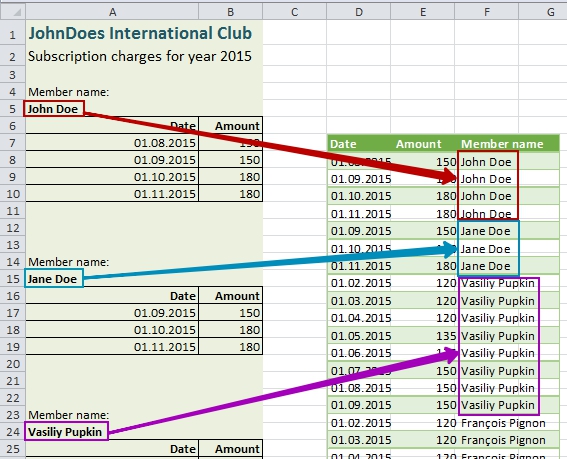
In this report we can see a standard header of what this document is about, and then information on each member’s charges. Each club member has own “table of charges” in this report, and each table precedes with two rows: pointer “Member name” and a member’ name itself.
In a sample report we can see four names: John Doe and Jane Doe form the USA, Vasiliy Pupkin from Russia and Francois Pignon from France (my apologies to monsieur Francois Dupont, but for me monsieur Pignon is already №1 due to beautiful comedies with Pierre Richard). Also please note that any coincidences to real people and clubs are accidental.
What we have to do is to make a flat table from the report:
Transfer values to a new column: things to do
Actually, we can name this operation as “partial column transfer”: we have to transform a part of column data into a values of new column(s).
There are several ways to make a flat table from this report: by Excel formulas, by VBA macro, or by Power Query in Excel 2010-2013 (“Get & Transform” in Excel 2016) or by Power BI.
Although transforming of this table in VBA could be very fast and scalable solution, our club cashier is in horror of any macro as he is convinced that it can steal his soul important information about club’ finances. So we will avoid a VBA solution for a while. An Excel formulas solution also looks very easy, but it has to be implemented “by hands” each time we got a report, and our cashier is too lazy to do it every month.
Ok, let’s start with Power Query. The sample workbook for this case could be downloaded from here.
May the Source be with you
In this case I will use named range for detecting our data area, but for practical purposes it looks more convenient to make a query to a source from another Excel file (we then have no need to define named range or make a table from a range).
So let us define the named range on whole report area and call it “Charges”. Just select report from cell A1 to last filled cell in column B and enter “Charges” in name field left to the formula bar.
(Actually I made a new sheet named “Charges” and applied named range on it)
First of all, let’s prepare data for following transformations. We need to clean all unnecessary data from report and make it more… usable.
- Open an “Empty query” in Power Query window.
- In formula bar enter = Excel.CurrentWorkbook()
- Click on “Table” left to our “Charges” name to expand.
Now we got a report in Power Query editor and can see the next expression in the formula bar: = Source{[Name="Charges"]}[Content] - Remove empty rows (we do not need them anyway): Main / Reduce rows / Remove rows / Remove empty rows. (I named this step as RemEmpty)
- Remove header rows: Main / Reduce rows / Remove rows / Remove first rows: 2.
Here we’ve got a little bit clearer view on data and can work it out:

A slightly cleaned source for future transformations
Let’s look closely at this data. This report has several significant features:
- unfortunately, each charges’ table has different rows count, so we can’t perform any transformation based on rows count
- fortunately, each table has the same structure
- each value we are looking for also has an exact place in Column1: it is located right before word “Data” and right after words “Member name:”
Whether or not, this data has the structure, and it’ll help us to “unravel the mystery” (and even in several ways!).
Give the query a name of “ChargesClean” and save it (“Save&Load to…” and make connection only). This query will be a source for our follow-up.
Transfer values “as in Excel”
What if we will solve this task in Excel “by hands”? The answer is a short formula for C4: = IF(A3=”Date”,A2,IF(A4=”Member name:”,””,C3)) . Then we just need to fill column C down with this formula, and result will be exactly what we are looking for: for each table we’ll got a corresponding person name right to column of charges and empty cells between tables. We can even shorten it: = IF(A3=”Date”,A2,C3) and get cells between tables filled with names form above table. Then we just need to replace formulas with values, remove rows between tables and inner headers.
We can do this in Power Query too. Just remember methods of relative references we made clear in my previous post: we need an “Index” column.
Let’s start.
- Right click on “ChargesClean query” – Make a link to it.
- Add column / Add index column / From 0. Rename this step to AddIndex (for simplicity)
- Add custom column with this formula:
=try if AddIndex[Column1]{[Index]-1}="Date" then AddIndex[Column1]{[Index]-2} else null otherwise null
Voila, we’ve got names in column right to amounts, and in first row of each small table. But we need names in each row of these tables. No problem: - Select “Custom” column and Transform / Fill / Down.
- Now we can remove “Index” column.
- Remove rows that we do not need any more by apply a filter to “Column2”: uncheck “null” and “Amount” values.
- Rename columns: “Column1” to “Date”, “Column2” to “Amount”, “Custom” to “Member name”.
- Change data types for columns: “Date” to type date, “Amount” to currency, “Member name” to text.
- Name our query as “ChargesR1C1” and save result to a sheet.
Here we finished.
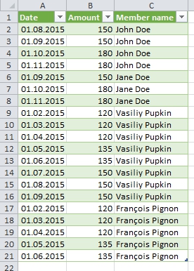
The result of a values transfer to another column
You can see that “partial transfer” works the same way in Power Query as it works in Excel: we just adopt Excel formula to ‘M’ language of Power Query.
But it is necessary to remember that using relative references in Power Query can clause a big performance decrease if a source is too large, so it is better to find another, more POWERful solution.
Use the Power, Luke
The other way to add columns to a table in Power Query is a merge of two tables. Really, if we would have two tables, one is our source and other with values we would like to add, and if we could find a key to link these tables, we can construct a new table with desired structure and data.
In the source (“ChargesClean” query) we have the only values which could play a role of a link key: it is the names of club members. Really, other data in the source is not distinct and cannot be used as identifier of data tables: only member name differs tables from each other. So, if we’ll got an appropriate table, we could link it to the source by this field.
Suppose that all names in the source are distinct, like MemberID, and let’s make a table to merge then.
- Make another query linked to a source: right click on “ChargesClean” query name in Queries Panel – make a link. Name the new query as “ChargesMerged”
- Remove all other data except names:
- Select “Column2” – filter – uncheck all except “null”.
- Remove “Column2”.
Now we have only one column with pointer in odd rows and names in even rows: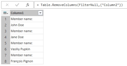
Almost ready
- Here we can filter this column to exclude the pointer “Member name:” or use trickier approach: remove alternating rows. To do this just use Main – Remove rows – Delete alternating rows, then enter 1 as row number to start, 1 as number of rows to delete and 1 as number of rows to skip.
Anyway, the result is the same, but I recommend just filter out “Member name:”.
- Although our sample has only different members name, it is better to make this list of names distinct (for a future purposes): Main – Reduce rows – Remove duplicates. Now we have a distinct list of members names and ready to merge this table with our source:
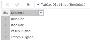
List of distinct names from report: ready to merge
(I named this step as “MakeDistinct”)
- Here goes a little trick (I’ll explain it a few rows later). Choose Main – Combine – Merge, select current query in lower part, select “Column1” in both queries and press “OK”. Don’t ever look at result, go to a formula bar and look at it:
1= Table.NestedJoin(MakeDistinct, {"Column1"}, MakeDistinct, {"Column1"}, "NewColumn", JoinKind.LeftOuter)
All we have to do now is replace first occurrence of previous step name with “ChargesClean” (or “Source”):
1= Table.NestedJoin(ChargesClean, {"Column1"}, MakeDistinct, {"Column1"}, "NewColumn", JoinKind.LeftOuter)And what we got there is:
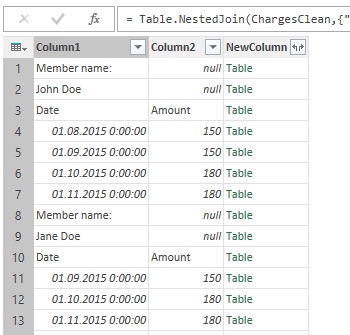
Merge done!
- Now expand “NewColumn” (press on “two-headed” row button near the column name), uncheck “use column name as prefix”, press “OK”:
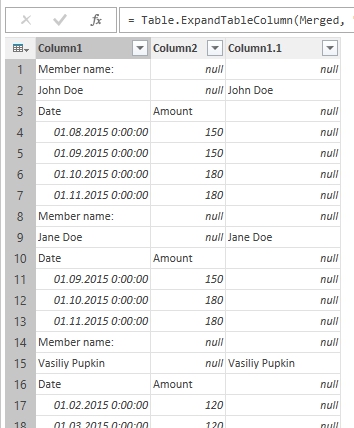
We are almost there
We can see that all member names from first column are doubled in the new column. The familiar table which need a standard make-up.
- Select “Column1.1” – Fill – Down.
- Apply filter on “Column2”: uncheck “null” and “Amount” (it leaves only numbers in this column)
- Change data types of result to date, currency and text accordingly.
- Rename columns to “Date”, “Amount” and “Member name”
We’ve got the same result as in Excel-style transformation, but without resource-consuming calculations for each row. Now we can “Save&Load” it to a new sheet.
Where is the catch?
Here I’ll explain the trick used in step 4, as promised.
When we make a merge from inside a query editor, we add other query to current. But for our goals we need current query to be added to our cleaned source with left outer join. Usual way to do this is either go to ChargesClean and perform merging in it, or make a new query by combining two other from “Workbook Queries” panel. But “ChargesClean” is used as a source in other query, so if we perform merging in it will cause an error in “ChargesR1C1”. And I don’t want to make any queries, so I just simulate this: I replaced first query name with the name of cleaned source. And as far as we used “ChargesClean” as a source to “ChargesMerged”, we can refer to the “ChargesClean” or to the “Source” step from “ChargesMerged”.
There also other way to link this source with a list of distinct names, but it is too much for a single post.
Credits: this post, being inspired by question on TechNet PowerQuery forum, was written under strong influence of excellent blog by Chris Webb, “’M’ is for (Data) Monkey” book by Ken Puls and Miguel Escobar and theirs blogs, the Gil Raviv blog on TechNet and a lot of other Power Query and Power BI pros & enthusiast.
Follow me:
Share this: